Descriptive and Explanatory Designs

Goals of Lifespan Developmental Science

Research methods are tools that serve scientific ways of knowing, and their utility depends on the extent to which they can help researchers reach their scientific goals. From a lifespan perspective, developmental science has three primary goals: to describe, explain, and optimize human development (Baltes, Reese, & Nesselroade, 1977; see Table 1.1). Because these goals are embedded within the larger meta-theory created by the lifespan perspective, they target two kinds of development: (1) patterns of normative change and stability; and (2) patterns of differential change and stability. When researchers say they are interested in understanding normative stability and change, they mean typical or regular age-graded patterns of individual change and constancy. When researchers want to understand differential development, they mean the different pathways that people can follow over time, including differences in the amount, nature, and direction of change. Moreover, researchers understand that some development entails quantitative changes (often called “trajectories”) and others involve qualitative shifts, such as the reorganization of existing forms or the emergence of new forms.

Description is the most basic task for all scientists. For developmental scientists, description involves depicting, portraying, or representing patterns of development in their target phenomena. This includes description of normative development, or typical quantitative and qualitative age-graded changes and continuities, as well as identifying the variety of different quantitative and qualitative pathways the phenomena can take. Explanations refer to explicit accounts of the factors that cause, influence, or produce the patterns of changes and stability that have been described. These are completely different from descriptions themselves. Descriptions answer questions like “what?” (i.e., the nature of the target phenomena), “how?” (i.e., the ways in which phenomena can change or remain the same), and “when?” (i.e., the ways in which these patterns appear as a function of age or time), whereas explanations focus on “why?”.

The goal of optimization refers to research and intervention activities designed to figure out how to promote healthy development (also referred to as flourishing or thriving) and the development of resilience. This task goes beyond description and explanation in two ways. First, in order to optimize development, trajectories and pathways must be identified as targets—targets that represent “optimal” development. These kinds of trajectories are often better than normative development, and so represent rare or even imaginary pathways, especially for groups living in highly risky environments. The search for optimal pathways reflects the assumption that individuals hold much more potential and plasticity in their development than is typically expressed or observed. The second way that optimization goes beyond description and explanation is that even when explanatory theories and research have identified all the conditions needed to promote optimal development, researchers and interventionists must still discover the strategies and levers that can consistently bring about these developmental conditions. One way to understand the difference between explanation and optimization is that, if explanations focus on the antecedents of a developmental phenomenon, then optimization efforts focus on the antecedents of these antecedents.

To learn more about these three goals, have a look at the expanded reading at this link.

Describe, Explain, Optimize [pdf]

The term design refers to “when,” “where,” and “how” data are collected, so the term can be used in three different ways.

Descriptive developmental designs refer to when data are collected. These included cross-sectional, longitudinal, and sequential designs. Explanatory designs refer to how and where data are collected, so they include experimental vs. naturalistic (or correlational) designs, and data collected in laboratory vs. field settings. As a result, designs combine all three of these features, for example, researchers conduct longitudinal field experiments, cross-sectional lab experiments, and naturalistic longitudinal field studies. In the next sections, these kinds of designs are explained in more detail.

Describing Development: Cross-Sectional, Longitudinal, and Sequential Designs

Developmental designs are ways of collecting data (information) about people that allow the researcher to see how people differ or change with age. There are two simple developmental designs: cross-sectional and longitudinal.

Why is it challenging to figure how people differ or change with age?

It is challenging because people’s lives are always embedded in historical time. As soon as a person is born, he or she is inserted into a specific historical moment. And, as the person ages and changes, society is changing right along with them. For example, if you were born in 1990, I know exactly how old you were when the Twin Towers fell, when the Great Recession hit, and when iTunes opened. From a research design perspective, we can say that peoples’ development is confounded with historical changes (that is, with the specific historical events and general societal trends that occur during their lifetimes). The problem with either of the simple developmental designs is that they do not allow clear inferences about (1) whether differences between age groups are really due to age or to historical differences, or (2) whether changes in people over time are really due to age changes or to historical changes. That is why lifespan researchers need to use designs that give them more information than simple cross-sectional or longitudinal studies do, such as sequential designs.

Can you remind me about the cross-sectional design?

A CROSS-SECTIONAL DESIGN collects information (1) at one point in time (one time of measurement) on (2) groups of people who are different ages.

Design for a cross-sectional (CS) study: (1) conducted in 1960, using (2) six age groups:

The good news about cross-sectional studies is that we get information about a wide range of age differences in a short period of time (one time of measurement), and we get information about differences between groups of people of different ages.

From a developmental perspective, however, the bad news about cross-sectional studies is that we don’t get any information about the thing we are most interested in, that is, change. Cross sectional studies provide no information (1) about how people change, (2) about pathways (or trajectories) different people take; or (3) about how earlier events or experiences predict later functioning.

What is the problem with cross-sectional designs?

The problem is that you CANNOT infer that differences between the age groups are the same as age changes.

Why not?

Because differences between age groups could be generational differences. What looks like age differences could really be cohort differences. Generational cohorts are groups of people who were born at the same time. They are sometimes just called “generations” and have been given labels, like the baby boomers, generation X, the millennial generation, and so on.

What are COHORT effects?

“Cohort effects” are the lifelong effects of belonging to a specific generation. They reflect the idea that being born at a specific time influences your development. Each of us has a series of experiences based on growing up during a specific historical period. Cohort effects also reflect the idea that specific historical events and trends have a different impact on people depending on how old they are. The Great Recession may have a very different effect on your development if you were 8 or 18 or 28 or 80. “Cohort effects” are the idea that people’s developmental pathways may differ based on the cumulative effects of these differences in experiences. If you want to learn more about different generations, you could watch this video about Generations throughout History (not required, bonus information).

What problem does that create for cross-sectional designs?

The problem is that the people in the different age groups also belong to different cohorts. In cross-sectional studies age is always confounded with cohort. Differences between the groups COULD be age differences or they COULD be cohort differences. You can see this confounding in the cross-sectional study depicted below. The participants who are 30 also belong to the 1930 birth cohort; the participants who are 40 also belong to the 1920 birth cohort, and so on. If we know the person’s age and the time of measurement, we can figure out their birth cohort.

Developmental researchers want to know if people differ according to their ages. But the fatal flaw with cross-sectional studies is that any differences between the groups in this design could be EITHER age differences OR generational (cohort) differences. Ages are completely confounded with cohorts (years of birth or generations). Any cross-sectional study could also be called an intergenerational study.

What is a LONGITUDINAL design?

It’s a study that examines (1) one group of people (2) repeatedly over multiple time points. Here is a longitudinal (LONG) study design that includes six times of measurement:

The good news about a longitudinal study is that it provides information about how people CHANGE or DEVELOP, as well as information about different people’s pathways or trajectories. It also allows researchers to see whether earlier experiences or events predict later outcomes.

BUT– are these really age changes?

Maybe, but they could also be historical changes. The fatal flaw with longitudinal studies is that changes in people over time could be EITHER due to age changes OR historical changes between times of measurement. As people age, the historical time they inhabit changes right along with them. Age and time of measurement are completely confounded, because all lives are embedded in historical time.

Can you see that age change is confounded with historical change in this longitudinal study? People who were 10 were also living in 1960, when they were 20, they were living in 1970, and so on. So, when people were changing from age 10 to age 20, the society they were living in also changed from 1960 to 1970. Therefore, people’s changes COULD be due to age (i.e., development), OR they could be due to historical changes over the times during which data were collected, or both.

If the simple developmental designs don’t work, what kinds of designs can developmental researchers use?

SEQUENTIAL designs are one good answer. They allow researchers to look at BOTH age changes and historical changes for multiple cohorts. There are many kinds of sequential designs. The one that we will learn about is called a Cross-sequential design. It provides the most developmental information in the shortest amount of time. It allows researchers to look at differences between people in terms of cohorts, and also to examine historical changes.

What is a CROSS-SEQUENTIAL design?

Cross-sequential designs combine cross-sectional and longitudinal designs. A cross-sequential study starts with a cross-sectional study that the researcher then follows up longitudinally for multiple measurement points. Here is a cross-sequential design (in green) that has 3 times of measurement, with 3 cross-sections (shown in the bottom row in yellow) and 8 longitudinal sequences (shown in the last column in blue).

The good news about a cross-sequential study is that this allows the researcher to compare longitudinal sequences across the same ages for different cohorts. So, for example, the researcher can compare what it’s like to go from age 20 to age 30 from 1960 to 1970 (LONG-2) with what it’s like to go from age 20 to age 30 from 1970 to 1980 (LONG-1). This way, the researcher can determine whether changes were due to age or tocohort differences.

This design also allows you to see if people who are the same age but from different cohorts are different from each other. For example, whether the 30-year-olds from the 1950 cohort are different from the 30-year-olds from the 1940 cohort or the 1930 cohort. If the age groups do not differ, you can zip the different longitudinal sequences together:

In this way, you can get imaginary long-term longitudinal information pretty quickly. That’s why the cross-sequential design is also called an “accelerated longitudinal design” or the “most efficient design.” The bad news about cross-sequential designs is that they are complex to conduct and to analyze.

Do SEQUENTIAL DESIGNS get rid of all the problems with developmental designs?

No, but they do allow you to look at them. It may be that age differences ARE generational differences or that age changes ARE shaped by historical changes.

If you are a contextualist, that’s the phenomenon you are actually interested in. However, you may need a historian to make sense of historical and cohort effects, and you may need to collect historical information as you go.

Explaining Development: Experimental and Naturalistic Designs

Description is the task of depicting, portraying, or representing patterns of development in the target phenomena, including patterns of normative age-graded changes and continuities, as well as the variety of different quantitative and qualitative pathways. In contrast, explanation refers to an account of the causes that together are sufficient to produce the patterns of changes and stability that we have described: What sets of factors cause, influence, or produce these different patterns of normative and differential change or stability over time? Explanation focuses on the weighty question of “Why?”.

Of the many features of research designs, the ones most relevant to explanation refer to the “where” and “how” of collecting data, so next we consider studies that use experimental and naturalistic designs conducted in the lab and field. In order to answer the causal questions of interest to lifespan developmental researchers, we want to create designs that allow us to make valid inferences about causes and effects as they unfold in the actual contexts of daily life. This is the information we will need to take with us into our optimization efforts. Let’s consider the four possible combinations of designs and settings (see Table below), one at a time.

LABORATORY EXPERIMENTS

What is an experimental design?

The defining features of an experimental design are twofold. The researcher (1) decides exactly what the causal agent (treatment) will be, and (2) determines who will get it (treatment group) and who will not (control group). So the challenges are also twofold: (1) to create a beautiful package of causal agents and (2) to ensure that the treatment and control groups are identical on everything but the treatment. Creating a plausible treatment that contains the causal ingredient is always an art, but researchers have become increasingly sophisticated in (1) isolating the putative cause by creating control groups who receive every single part of the experience of the treatment group except the specified causal agent; and (2) ensuring that control groups are identical to the treatment group on preexisting attributes, both known (which can be equated via matching or controlling for measured attributes) and unknown (which can be equated via random assignment; Campbell & Stanley, 1963; Shadish, Cook, & Campbell, 2002).

In many design classes, you will learn that the best design (and some will say the only design) for demonstrating causality is the experiment. So, for some researchers, the experiment (and not the time machine) is considered the “gold standard.” And, in the olden days, it was often assumed that experiments only happen in the laboratory, so experimental designs and laboratory settings are often merged in students’ minds. So let’s take a minute to consider experiments in labs.

Do labs provide advantages for detecting causality?

Indeed they do. They cannot be beat for settings in which the researcher has complete control over both key design features. Researchers can ensure that assignment to experimental or control conditions is completely random; and they can guarantee that the hypothesized causal variable is administered exactly as prescribed. Labs also provide very clear lines of sight on our phenomena—both potential causes and potential effects.

Do lifespan developmental researchers care about random assignment?

Yes. Huge problems are created by the fact that in the contexts of daily life people are not randomly assigned to causal conditions—there are particular personal characteristics that belong to the people who get in the way of particular causal forces, or who participate in them directly. And so, if we are going to distinguish pre-existing conditions that launched someone on a particular developmental trajectory from the causal factors that we are interested in discerning, we have to create groups that are “the same on everything” before we start our causal show. Randomized assignment is one strategy to accomplish this, as well as its more systematic options, such as block randomization (randomly assigning different categories of people), matching, propensity score matching, and so on.

Why are we so excited about exact control of the causal factor?

Well, that’s the magic of experimental designs. The researcher is like the fairy godmother who waves her wand and introduces the potentially new future for the treatment group. So the researcher knows that the treatment group got the potential causal factor, and how much of the factor, and so on. And then the researcher has approximately a bazgillion control groups, who got shades of everything but the hypothesized active ingredient. These can be very creative, the control group with nothing, with only attention, with a visit to the lab but no causal factor, with a causal factor that looks like the actual causal factor but really isn’t. Remember “placebos,” which were added to drug trials so that the control group even gets the experience of taking a pill?

NATURALISTIC LAB STUDIES

Are there lab studies that do not involve experiments?

Yes. They are called naturalistic lab studies because researchers bring participants into the lab setting, but do not administer a dose of a potential causal agent.

What would be some uses for naturalistic lab studies?

One important use is to measure constructs that you can’t capture outside of the lab. There are some phenomena of great interest that are not visible without specialized instrumentation or procedures that can be administered only in the lab setting. All manner of neurophysiological constructs can only be measured in the lab using complex equipment, like fMRI, as well as the assessment of internal states and capacities, like executive function or delay of gratification or implicit bias. Researchers can work with their participants in the lab in order to make these internal processes more visible. One great example is the “talk aloud protocol,” in which individuals (even children) are trained to narrate their mental processes as they work on a task or watch a demonstration. These protocols provide stream of consciousness information that would not be accessible in any other way.

A second important reason researchers might turn to lab settings is to create conditions where they can trigger and then observe interactions that are relatively rare in field settings. For example, research on learned helplessness often brings children into controlled settings where researchers can watch them work with solvable and then with unsolvable puzzles, mazes, and concept tasks, while monitoring their strategies, efforts, and actions over time. (And, of course they always end with success experiences.) Another example is the Strange Situation in which researchers trigger the attachment system in the living-room-like lab setting, by sending in a stranger and asking the caregiver to leave, and then observing the child’s actions.

These experiences are both rigorously standardized and intuitively compelling for participants. They can simulate transgressions (e.g., when a child hears a child in the next room knock over her block creation), competitions (e.g., when two children are playing a videogame and one messes up), exclusion (e.g., when a child is left out of a ball tossing game), and so on. Such standardization creates comparability among participants. It allows researchers to be sure that their differential responses are not due to differential provocations, but to their individual reactions to identical experiences.

In all these cases, naturalistic observation may seem more desirable, but social processes can be impossible to tease apart as they unfold in daily contexts. For example, mastery-oriented children run into fewer tasks they cannot solve than helpless-prone children and so it is harder to catch them in failure situations, and in schools teachers do not assign impossible tasks, and so observers could go for weeks without seeing their phenomena. And, by the way, after about five years of age, kids are busy trying to hide their true reactions to negative events (a phenomenon called “masking”), which makes it harder for observers to actually detect undesired states (like anxiety or boredom) in the field. In fact, precisely because people and their contexts are so intertwined, we sometimes bring our participants into the lab to see what they can do without the scaffolds or interference of social partners.

What are the main advantages of experimental and naturalistic lab studies?

Their claims to fame are control and precision. Because we have exact control of the causal factor and exact control over who receives it, we can make unambiguous causal inferences. These may be especially appreciated when we are trying to untangle the directions of effects in reciprocal proximal processes or transactions. Moreover, we have precision in our measurement or observation of the targets—both causes and effects. We can see below the surface (into neurophysiology or cognitive functioning). We can even trigger phenomena that are rare or hard to see in the wild, and record their details using our video cameras or talk aloud protocols.

What are the disadvantages of studies conducted in lab settings?

Well, for lifespan developmental researchers, they have some pretty serious limitations. Let’s think about three big ones. First, labs and fields are more than settings to us. They are contexts. And contexts are not just geographic and architectural locations, in the sense that you can simply pick people up and “set” them down in new places. Contexts have tentacles that reach out and wind themselves around people, and people have roots that reach down into places. They are connected, mutually created, interpenetrated even, so that our most likely causal forces, our proximal processes, cannot even be constituted when we look at only one without the other. When researchers split the child from his or her context, it destroys the phenomenon itself, like removing the heart from the body in order to see how it works. You can’t. Once you remove it, it doesn’t work anymore. So we worry that lab studies can alter or distort our phenomena.

So developmentalists don’t conduct research in laboratory settings?

Not at all.  Contextualists are just very wary about the idea of the “setting” and very aware of what is lost by leaving the “scene of the crime,” that is, the contexts of daily life. The “field” is an intrinsic and crucial part of the target we are trying to understand, and if we are going to bring our whole phenomenon into the lab, we have to know all the relevant elements of the context and effectively simulate them in the lab. Otherwise, this kind of distortion can be a threat to internal validity.

What is the second limitation of laboratory studies?

Second, we assume that all our causal factors are embedded in contexts and shaped by them. Instead of thinking about the lab as a place where researchers can get more pristine information about their target phenomena (the child and their behavior), the lab has come to be regarded as one context with its own attributes (e.g., novelty) and set of social partners (i.e., the experimenter) that are exerting their own effects on the child. So if we are looking at the functioning of proximal processes in the lab, we can be sure that the lab context is shaping then, which means we can’t be sure that they actually operate the same way in the contexts of daily life. As a result, we always have to admit that any causal links we may have created in the lab have to be couched as “can cause” our target and not as “does cause” our target. We have to wait and see if these same processes are operating in the actual contexts that form the natural microsystems for our participants. Otherwise, this kind of artificiality can be a threat to external validity.

Third, the time span over which developmentalists assume that causal effects accumulate cannot be easily simulated in the lab. The causal processes of interest to developmentalists unfold over months and years and decades, across multiple contexts, so although we can use the lab to measure the long-term effects of causal factors by bringing our participants back to the lab as many times as we want to, if we want to actually lookat the causal processes having their effects over months or years, it will be difficult to achieve that in the lab setting.

And are there corresponding disadvantages with experimental designs?

Well, for some developmentalists, they do have a fatal flaw. As noted by many methodologists, the seemingly insurmountable problem with experimental designs is that it is not possible to randomly assign or manipulate the causal forces that are of biggest interest to developmentalists. No one can randomly assign their participants to a particular age group (“I have flipped a coin and you will be in the five-year-old group” “Oh no, I wanted to be 10!”) or to a particular cohort or developmental history.

In fact, most of the causal factors that are of interest to us can’t ethically be manipulated at all—the happy single-parent family versus the unhappily married parents, the delinquent peer group versus theatre-obsessed friends, school failure versus success, peer rejection versus popularity, high stress reactivity, dangerous neighborhoods, or height. Before you ask, we will just add that this same issue applies to all areas of psychology. Many applied problems cannot be manipulated—divorce, PTSD, dangerous job conditions, psychopathology, work-family conflict, serious medical diagnosis, intimate partner violence, and so on. So there are serious limitations to how much experimental designs can help applied researchers study the conditions and causes that matter most to them.

FIELD EXPERIMENTS 

Wait! What about field experiments designed to promote development?

Yes, indeed. And these field experiments can even be conducted as randomized controlled trials (RCTs; Shadish & Cook, 2009). And, yes, we can ethically study any old target we please as long as we are trying to promote development—to remediate unfavorable developmental trajectories, to maintain resilient ones, and in general to prevent adverse and promote healthy development.

What are randomized controlled trials?

As you may know, this methodology was borrowed from clinical trials of medical treatments, and it is cool in many ways. It has time in its design, which is always welcome news to developmentalists. RCTs compare (at least) two groups who should be equivalent to each other (based on random assignment), one of which has received the treatment and the other a placebo, so that researchers can examine the effects of the treatment over and above the effects of knowing that one is being treated. Then after a sufficient amount of time for the treatment to do its work, changes in the treatment and control group can be compared over however many time points the design includes. In recent decades, RCTs in field settings have become de rigueur for settling causal claims about “evidence-based” practices, programs, and policies. RCT field experiments provide a standard of proof that has made them essential to both the scientific community and to applied decision makers and stakeholders (e.g., see the What Works Clearinghouse). 

Do these kinds of studies have certain advantages?

Indeed, they do. Some researchers see field experiments as the best of both worlds. On the one hand, studies get to keep all the compelling features of experimental designs that are so helpful in making unambiguous causal inferences. But on the other hand, we have escaped from the lab setting and returned to the contexts of everyday life, so they generally evince higher authenticity and external validity. Often treatments are even administered by natural social partners in everyday contexts. Parents, teachers, bosses, coaches, or mentors receive systematic training and then bring their newly acquired attributes back into the settings of homes, classrooms, and workplaces, where researchers can determine whether they subsequently change the proximal processes and the development that takes place there.

Are there disadvantages to field experiments?

Many researchers consider RCTs to be “the gold standard,” but they have three important limitations for developmentalists. First, the very thing we like about them—getting out of the lab and into the field—can make the administration of the causal factor somewhat messy. We lose some of our beloved control and precision. Especially if researchers decide that the treatment (often an intervention program) will be administered through intermediaries (like teachers or caregivers or social workers), it can be a giant headache. A whole area of study, called “implementation research,” focuses on “implementation fidelity”—or how to make sure that participants actually make contact with the active ingredients of the potential causal factor.

Moreover, in the real world, participants can drop out of the treatment (e.g., the teacher or parent training) any time they want, but they do not drop out of the treatment group in our design. To maintain the equivalence between treatment and control groups accomplished by our initial random assignment, participants cannot voluntarily switch groups—or we have suddenly introduced bias. So the treatment group is often labeled the “intent to treat” group, meaning that participants were initially assigned to this group, even if they end up receiving no treatment whatsoever. It’s like doctors who send the treatment pills home with their patients and then hope for the best, but never get to count the pills that are left in the bottle at the end of the trial. If patients do not improve, they can’t really say whether the drug didn’t work or whether the patients just didn’t take their pills. Unsettling from a causal inference perspective.

A second limitation, and one that field experiments share with lab experiments, is that they cannot tell us what caused these unhealthy pathways of development in the first place, any more than studying aspirin can tell us what causes headaches or how to prevent them. So additional work will always be needed to fill in the causal puzzle of the factors that contribute to and maintain non-optimal development or lead to psychopathology. Such studies would be essential to prevention efforts.

Third, RCTs (in both lab and field) have inherent limitations in providing causal explanations. At the end of the day, the only thing that this design can tell you is “yes” or “no.” That is, the only information it yields is whether the two groups– treatment and control– are different. You can add many features, for example, many indicators of disease or health, you can measure dosage and its effects, over several time periods, and so on. However, developmentalists would say that, after all this work, the only thing we have in our hands is a causal description but not the thing that we most want, that is, a causal explanation. For the drug companies, everything they want to know about causal explanations is contained in the drug itself. To the extent that they care about how the drug works, its mechanisms of effects have already been studied (and of course, we take many drugs that are effective, but whose mechanisms of effects are unknown).

But as developmentalists, our interventions contain hundreds of potential active ingredients. And so we want to poke our heads under the hood and look all around, watching the cogs engage and the wheels turn. We want to watch the tennis game or the dance, and see who is hitting the ball the hardest and how the players adapt to each other’s style over time and who is playing the music. In other words, we are on the trail of causal explanation and so we can’t really be satisfied with “yes” or “no.” We will forever be asking “Why?” or “Why not?” and especially “How did that work?”. So we will always be supplementing experimental and lab studies, and even RCT studies, with studies using designs that can provide us with more complex process-oriented accounts of the multiple causes of differential developmental trajectories and transformations.

Take Home Messages about Different Explanatory Designs and Settings

All designs, including experimental lab and field designs, have advantages and disadvantages (see Table). Your job is to conduct each kind of study using the very best methods available (that’s the “looking” part of a scientist’s role) and then to keep straight on what you can and cannot see (that’s the “thinking” part of a scientist’s role). That way, you will learn what there really is to be learned using experimental designs, and then start longing for what can be seen using alternative designs that provide other lines of sight.

NATURALISTIC FIELD STUDIES

What we appreciate about naturalistic field studies is obvious from the limitations we encountered with lab and experimental designs: In naturalistic studies we can examine the effects of potential causes we can’t possibly administer (e.g., maltreatment, ability tracking, peer rejection). Moreover, we can watch these processes operate in their authentic multi-level contexts, and we can follow them for months and years.

But aren’t experiments the only way to show causality?

Yes, experiments can provide important evidence of causal processes. But let’s consider the kinds of causal evidence that can be provided by naturalistic studies. 

Are we talking about correlational studies? Because we know for a fact that “correlation does not prove causation.”

Right, it is correct that correlation by itself does not prove causation. But let’s take a minute to understand why this is true, and then to see whether there are some things that researchers can do to improve the designs of their studies so that naturalistic studies, using more than correlations, can provide evidence about causes. Because, remember—correlation may not prove causation, but causal processes do generate correlations: Since causes produce effects, effects covary with their causes. In fact, this covariation is a defining condition of causality (see box). As a result, correlations (or covariation or contingencies, however you want to label them) may be the smoke that leads us to our causal fires. The problem is that many things besides causation lead to correlations, and so we have to work hard to decipher the causal evidence among all the other kinds of covariation information we are examining.

Okay, can you break down the reasons that correlations do not prove causation?

Yes, let’s start with a consideration of a typical correlation between two variables, and let’s pick variables that tap constructs we think could be causally connected, say, teacher involvement and student engagement (see figure below). Let’s say that in this research we get a robust correlation between good measures of both variables. Why can’t we conclude that teacher involvement influences student engagement? There are two main reasons. First, as also shown in the figure below, the connection between these two variables could be due to a reciprocal causal effect, in which student engagement influences teacher involvement. This direction of effects is conceptually plausible, since more engaged students could attract more positive teacher attention whereas more disaffected students could lead teachers to withdraw or treat students more harshly. Of course, the correlation could be due to both feedforward (i.e., teachers’ influences on students) and feedback (i.e., students’ influences on teachers) effects.

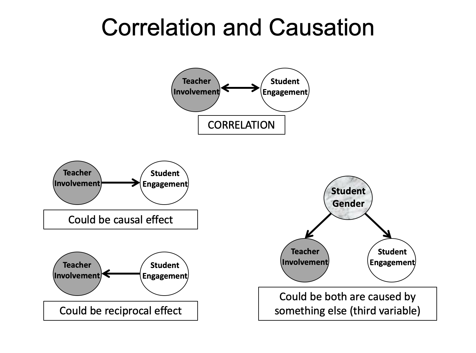
The second possibility is that there is no causal effect at all between these two variables (forward or backward). Instead, they are both actually produced by a completely different cause (the ominously named “third variable”); and they covary only because they are both effects from the same cause. In our example, also shown in the figure, we selected students’ gender as our third variable because gender is a plausible cause of both variables. In general, girls are more engaged and teachers show more involvement with them, whereas boys generally tend to be less engaged and teachers show less warmth toward them. In this scenario, as in all other scenarios involving concurrent correlations, there are a very large number of third variables (alternative causes of both) that could be in play—it could be achievement (engaged students perform better in school and teachers attend more to high performing students) or social class or student sense of relatedness—as well as a large number of third variables that we can’t immediately imagine. So in naturalistic designs, we use the term “third variable” as shorthand for all the alternative causal explanations that could underlie the connections between our hypothesized antecedent and its possible consequence.

Is there anything we can do to help solve these problems?

Yes, including time in the design of our naturalistic studies helps us out quite a bit.

What do you mean by “adding time” to a design?

When we say we are “adding time” to a design, we mean that we are adding “occasions” or “times of measurement” or “repeated measures” to a design.

Like in a longitudinal study?

Yes, but maybe the most general description is “time series” because the design includes a series of different times of measurement.

What are the advantages of adding time?

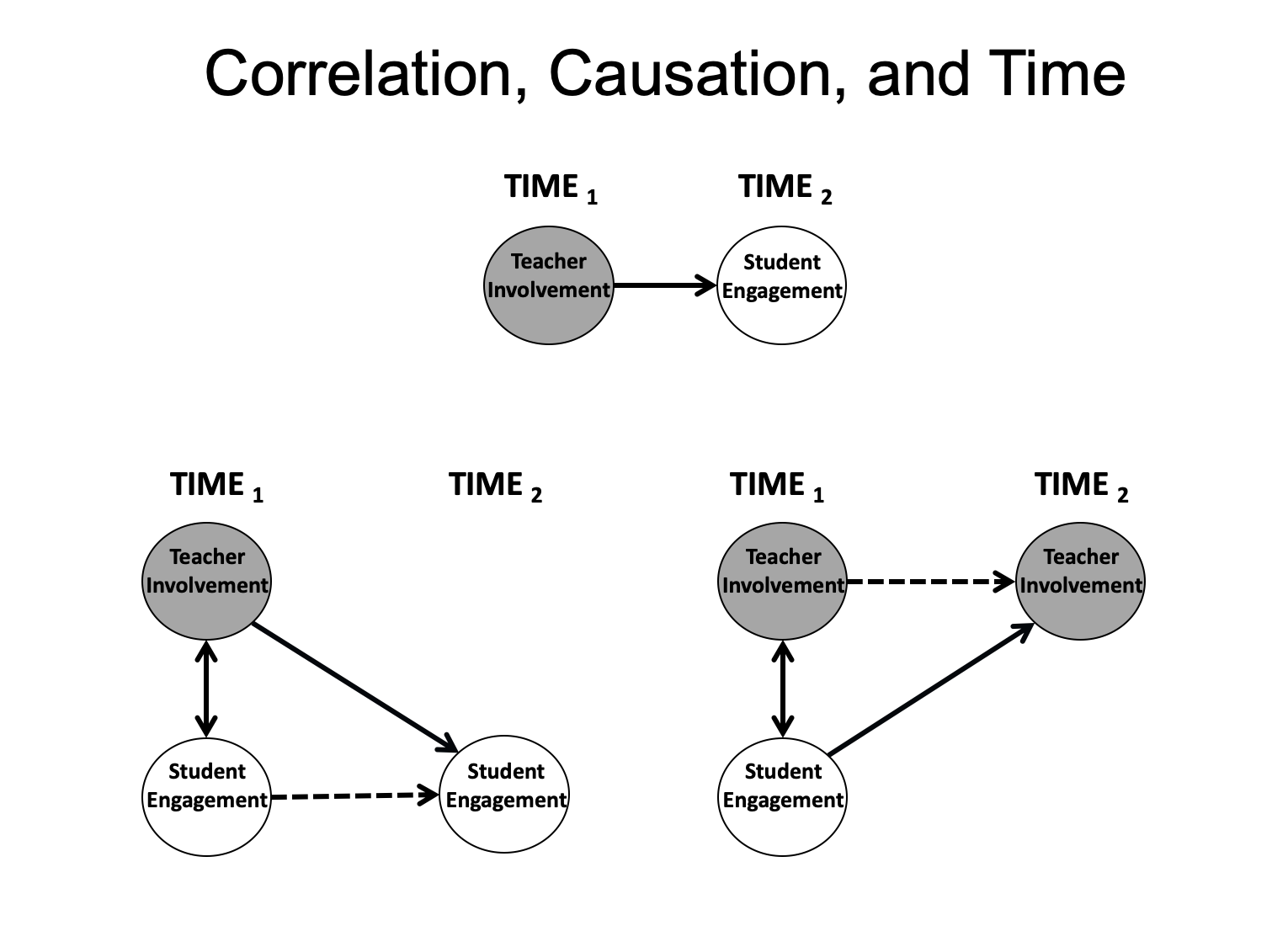
Let’s say that we add just one more time of measurement, so we have two waves in our study. The first advantage is that now we have a way to check the first condition of causality, namely, that causes precede their effects. So we can check out a time-ordered correlation. Continuing with our example, with time in the design, we can look at whether the potential cause at Time 1 predicts the potential outcome at Time 2. This is depicted in the figure below. So we are excited to be able to use the word “predict” correctly to describe our correlation. However, this is still just a zero-order bivariate correlation, so it does not allow a causal inference—it still has all the problems with those dreaded “third variables” or alternative causal explanations. But we can use our two time points to start looking at how our target outcome is changing from Time 1 to Time 2 and to see whether those changes can be predicted from where each person was on the potential cause at Time 1.

So what do we like about this kind of design?

We get to look at developmental trajectories as our outcomes (and if we add more time points, they will look more like trajectories), we are looking directly at individual differences in trajectories, and we are looking at predictors of individual differences in those trajectories. So, in our example, we can ask, “Does teacher involvement at the beginning of the school year predict changes in students’ engagement from the beginning to the end of the school year?”. And if the empirical answer is “yes” (i.e., the antecedent is a significant predictor of change from Time 1 to Time 2), we can say things like “Students whose teachers were warmer and more involved with them at the beginning of the school year, also showed increases in their engagement over the school year; whereas students whose teachers were less involved with them at the beginning of the school year, showed corresponding declines in their engagement as the year progressed.” This is a descriptive statement, but it is consistent with a causal hypothesis.

Any other advantages?

Yes. We can also, using the same design, look at the “reciprocal” predictions, in that we can take our antecedent variable and examine how it changes from Time 1 to Time 2, and see whether the variable we had been thinking of as a consequence (which we now consider as a possible antecedent) predicts these changes—see the figure above. In our example, we would be asking “Do students’ initial levels of engagement at the beginning of the year predict changes in how much involvement their teachers provide them over the year?” And, if the empirical answer is “yes,” we can say things like “Students who were more engaged in fall experienced increasing involvement from their teachers as the year progressed, whereas students who were initially higher in disaffection experienced declines in their teachers’ involvement from fall to spring.” One of the most important things about a design with two points of measurement (remember, we just added one more point) is that it allows researchers to begin to pull apart the different directions of effects. A concurrent correlation contains information about both directions of effects, which cannot logically be untangled, but the two analyses that we just ran can get the job done—the first looks at the feed forward prediction of teacher involvement on changes in subsequent student engagement, whereas the second looks at the feedback prediction of student engagement on changes in subsequent teacher involvement. So the answers to the questions posed by these two sets of analyses could be different—we could get two “yes”s or two “no”s or one of each. And if we get two “yes”s, we have the possibility of a feedback loop, which feels like we are getting some hints about potential dynamics in the system.

What about all those pesky third variables, those alternative explanations?

Well, we have good news and bad news about them.

What is the good news?

The good news is that we have reduced them some. If you start thinking about the third variables in the concurrent correlation in our illustration, that is, all the factors that are positively correlated with both teacher involvement and student engagement, an enormous number come to mind (e.g., achievement, SES, supportive caregivers, IQ, a sense of relatedness, and so on). And here is the kicker, these are only the ones we can imagine, there are also unknown confounders. However, when we include in our design and analyses intra-individual change over time, we are using people as their own controls. This means that out of our potential consequence at Time 2, we are taking each participant’s starting value of the consequence at Time 1, which has in it by definition everything (known and unknown) that led up to the consequence at Time 1 (e.g., achievement, SES, supportive caregivers, IQ, a sense of relatedness, and so on) as well as all the unknowns that created or predicted the consequence at Time 1.

So, for example, if we think that achievement is a possible alternative causal explanation for the zero-order correlation between teacher involvement at Time 1 and student engagement at Time 2 (meaning that high performing students are more engaged and teachers pay more attention to them), when we control for student engagement Time 1, we take out all of the achievement that was responsible for engagement up to that point, so we have controlled for that as a potential confounder. By controlling for the same variable at an earlier point in time, we have scraped off all the known and unknown predictors of engagement up until Time 1 that could be a potential confounder, or a plausible pre-existing difference, or an alternative causal chain.

So then what is the bad news?

The bad news is that the notorious third variables are not completely eliminated. Since we are still looking at a kind of correlation—specifically the correlation between teacher involvement at Time 1 and changes in student engagement from Time 1 to Time 2–  we are still on the hunt for possible alternative causes of both. Remember, before we were looking for things that were correlated with both teacher involvement and student engagement, but now, with this design, we can narrow our candidates for third variables down to those that are correlated with both teacher involvement and changes in student engagement. 

What should we be thinking about in adding time to our study design?

Let’s start with some basic questions that we almost never know the answers to—What are the right windows and the right time gaps between measurement points? We ran into this problem, called “time and timing” (Lerner, Schwartz, & Phelps, 2009), in the chapter on descriptive longitudinal designs, when we had to pick the developmental window (time) over which we thought our target change was likely to occur, and then decide on the spacing between measurement points (timing) needed to capture its hypothesized rate and pattern of change. In descriptive designs, we ask these questions about the developmental outcomes, but in explanatory designs, we also ask them about the causal process: “During what developmental window (time) are our target causal processes likely to be active?” and “What spacing (timing) should we use to capture the rate at which this causal process is likely to generate its effects (both feedforward and feedback)?”. For example, if we are thinking about teacher involvement and student engagement, it seems like the beginning of a new school year would be a good moment for them to be calibrating to each other (time), but how long would that take (timing)—a week, a month, six weeks? Who knows? One rule of thumb is to use more measurement points than you think you will need, so you can look over different time gaps for your possible process.

What do you mean “more”? Weren’t we excited to be adding just one more time of measurement?

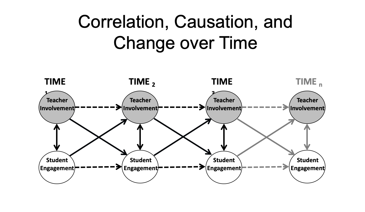
Well, two is qualitatively better than one, so that’s good. But more really is merrier. Additional times of measurement allow researchers to look at these predictors of change across additional time gaps, for example, from a predictor at Time 2 to changes from Time 2 to Time 3 (as depicted in the figure). Multiple time points also open up a new world—one filled with trajectories of mean level change as the outcomes of our causal processes.

A first step in this direction has been referred to as a “launch” model because it tries to examine whether an individuals’ initial levels on an antecedent can predict the individuals’ trajectory on the target consequence. The term “launch” is used because such a model assumes that the initial levels of the potential causal variable may act like a catapult or rocket launcher to create the direction and angle of change in the object that is hurled, that is, the target outcome.

Can we even use these designs to look at how changes in our antecedents predict changes in our outcomes?

Yes, these have been called “change-to-change” models), but you can’t really use the word “predict” to describe these connections. They are actually like correlations between growth curves, and then we land back in our concurrent correlations puddle—where we still don’t know who is preceding whom. So it would probably be better to look at the connections between time-lagged growth curves, for example, the connections between a growth curve from Time 1 to Time n to predict an outcome from Time 2 to Time n+1. Then you could also look at reciprocal change-to-change effects by switching around your antecedents and consequences. Just like with the designs that incorporate only two measurement points, these two analyses can provide different estimates of the connections between the different portions of the growth curves.

What is happening with all our third variables in these analyses?

We can control for them, but it may be more interesting to look directly at their effects, by organizing our data into a “niche” study, where we look at the connections we are interested in for subgroups of children—for boys or girls separately or for students high or low in achievement. If the connection between teacher involvement and student engagement is due to gender, it will disappear when we look at boys and girls separately. As you know, looking directly at the developmental patterns of different groups is more consistent with a lifespan developmental systems perspective, which holds that development is differentially shaped by the characteristics of the people and their contexts.

These design ideas for naturalistic studies seem much less systematic than the strategies we learned about for experimental studies.

Yes, it can sometimes feel like the wild west out here on the frontier where we are trying to extract valid causal inferences from naturalistic studies. But keep in mind that you are not alone. Researchers from many other disciplines, like epidemiology, sociology, and economics (e.g., Gangl, 2010; Heckman, 2008), are also developing useful methods for tracking down causal processes, because they can no more create controlled experiments– in which they crash stock markets or start epidemics or shift social mores—than can developmental scientists. As part of this search, they are uncovering an important set of tools for causal inferences in the careful application of sound statistical methods (e.g., Madigan et al., 2014; see box).

Take Home Messages for Naturalistic Field Studies

We would highlight four.

1. The first is a resounding “Yes!” to the question of whether naturalistic field studies can contribute to rich causal accounts of development. These are studies that contain everything you want to know about your target phenomenon, so it is worthwhile to figure out how to decipher that information in ways that yield valid causal accounts.
2. The second take home is a resounding “Whoa!” because the ways that causes likely operate in the complex dynamic system of which our target phenomenon is a part can be truly mind-bending. So we need to pause and get our meta-theoretical glasses firmly on our noses before we start sifting through designs and strategies.
3. Third, our most trusty tool is time itself—the times of measurement in longitudinal and time series designs, the time windows over which we choose to hover, and the timing (spacing) of our measurements so they map onto the pace of our causal processes.
4. Our final take-home is that the search for design ideas for wresting causal information out of naturalistic field studies will take you into some beautiful and uncharted territory. When you encounter a complex problem (like historical embeddedness or cohort effects), your immediate reaction may “How do I avoid this problem?” or “How do I solve this problem?” But instead of resorting to coping, we would encourage you to react with curiosity. In other words, the best advice that lifespan developmental researchers can give themselves is always “Don’t ignore. Don’t evade. Turn around and look.” These are not methodological problems you have encountered. They are messages from your target developmental phenomena. And, if you have ears to hear, you can learn a great deal by walking directly towards them.

Take Home Messages for the Goals of Developmental Science and Descriptive and Explanatory Designs

Take home messages are also contained in the summary tables for the three goals of developmental science, and the tables describing (1) cross-sectional, longitudinal, and sequential designs, and for (2) experimental and correlational designs in the laboratory and the field. For the designs, we would like you to be able to define each one, identify the advantages and disadvantages of each, and discuss when it would make sense to use each of them in a program of research. Be sure to revisit the concept of converging operations— it helps pull together the idea that the strengths of each design can help compensate for the weaknesses of other designs!

Supplemental Materials

• This chapter discusses the use of qualitative methods in psychology and the ways in which qualitative inquiry has participated in a radical tradition.

Kidder, L.H., & Fine, M. (1997). Qualitative inquiry in psychology: A radical tradition. In D. Fox and I. Prilleltensky (Eds.) Critical psychology: An introduction (pp. 34-50). Thousand Oaks, CA: Sage.

• This article discusses the approach and method of Youth-led Participatory Action Research and implications for promoting healthy development.

Ozer, E. J. (2017). Youth‐led participatory action research: Overview and potential for enhancing adolescent development. Child Development Perspectives, 11(3), 173-177. doi:http://dx.doi.org/10.1111/cdep.12228

• The following article examines systematic racial inequality within the context of psychological research.

Roberts, S. O., Bareket-Shavit, C., Dollins, F. A., Goldie, P. D., & Mortenson, E. (2020). Racial inequality in psychological research: Trends of the past and recommendations for the future. Perspectives on Psychological Science, 1745691620927709.

References

Baltes, P. B., Reese, H. W., & Nesselroade, J. R. (1977). Life-span developmental psychology: Introduction to research methods. Oxford, England: Brooks/Cole.

Campbell, D. T. & Stanley, J. C. (1963). Experimental and quasi-experimental designs for research. Boston: Houghton Mifflin.

Case, R. (1985). Intellectual development. New York: Academic Press.

Eccles, J. S., & Midgley, C. (1989).  Stage/environment fit: Developmentally appropriate classrooms for early adolescents.  In R. Ames & C. Ames (Eds.), Research on motivation in education (Vol. 3, pp. 139-181).  New York: Academic Press.

Eccles. J. S., Midgley, C., Wigfield, A., Buchanan, C. M., Reuman, D., Flanagan, C., & McIver, D. (1993). Development during adolescence: The impact of stage-environment fit on adolescents’ experiences in schools and families. American Psychologist, 48, 90-101.

Gangl, M. (2010). Causal inference in sociological research. Annual Review of Sociology, 36, 21-47.

Heckman, J. J. (2008). Econometric causality. International Statistical Review, 76(1), 1-27.

Lerner, R. M., Schwartz, S. J., & Phelps, E. (2009). Problematics of time and timing in the longitudinal study of human development: Theoretical and methodological issues. Human Development, 52(1), 44-68.

Madigan, D., Stang, P. E., Berlin, J. A., Schuemie, M., Overhage, J. M., Suchard, M. A., … & Ryan, P. B. (2014). A systematic statistical approach to evaluating evidence from observational studies. Annual Review of Statistics and Its Application, 1, 11-39.

Mill, J.S. (1843). A system of logic. London: Parker.

Shadish, W. R., & Cook, T. D. (2009). The renaissance of field experimentation in evaluating interventions. Annual Review of Psychology, 60, 607-629.

Shadish, W. R., Cook, T. D., & Campbell, D. T. (2002). Experimental and quasi-experimental designs for generalized causal inference. Wadsworth Cengage learning.