4 Vignette 4: Fluvial sediment transport
Adam Booth
THEORY
Movement of sediment at the bed of the river occurs when the shear stress exerted on the bed by the flowing water above is sufficient to accelerate the sediment (i.e. driving force exceeds resisting force). To calculate what flow conditions are necessary for this to happen, we first need to know what the shear stress acting on the bed is. We will assume steady flow so that the shear force acting on the bed must be equal to the net fluid force driving the flow of a theoretical column of water across each patch of the bed (Figure 1).
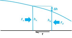
Since the shear stress is ultimately what we are interested in, we will define shear force acting on the bed, [latex]F_b[/latex], first in general terms as the product of the shear stress and the area of the bed,
Equation 1:
[latex]F_b=τΔxΔy[/latex]
where [latex]τ[/latex] is the shear stress [M L-1 T-2], [latex]Δx[/latex] is length of the water column being considered in the direction of flow [L], and [latex]Δy[/latex] is the cross-channel width of the column [L]. Similarly, fluid force, [latex]F_f[/latex], on either side of the column is equal to the average fluid pressure multiplied by the cross-sectional area,
Equation 2:
[latex]F_f=\bar{P}A_f[/latex]
where [latex]\bar{P}[/latex] is average pressure [M L-1 T-2], and [latex]A_f[/latex] is the cross-sectional area of the flow [L2].
Pressure is linearly proportional to depth from the surface of the flow, so we know the average pressure is the same as the pressure at half the depth, [latex]\bar{P}=ρgh[/latex], where [latex]ρ[/latex] is fluid density [M L-3], [latex]g[/latex] is acceleration due to gravity [L T-2], and [latex]h[/latex] is the depth of the flow [L].
Cross-sectional area of the flow is simply [latex]hΔy[/latex], so substituting that along with the definition of average fluid pressure into Equation 2 and simplifying, we can write the fluid force as:
Equation 3:
[latex]F_f=\frac{1}{2}ρgh^2Δy[/latex]
Since the depth is different on the upstream and downstream sides of the water column, we must subtract them to get the net force across the patch of bed beneath the column.
Note that this difference in fluid force is caused by the water surface having different elevations, so it is the surface slope of the fluid that drives the flow, rather than the slope of the bed. In some cases, water surface slope and bed slope may be the same, but in many others, such as deltas, they typically are not.
The magnitude of this net fluid force must balance the resisting force since we assumed steady flow, so we can set Equation 1 equal to difference between the upstream and downstream fluid forces:
Equation 4:
[latex]τΔxΔy=F_u-F_d[/latex]
Substituting Equation 3 for the fluid forces gives:
Equation 5:
[latex]τΔxΔy=\frac{1}{2}ρgh_u^2Δy-\frac{1}{2}ρgh_d^2Δy[/latex]
which simplifies to:
Equation 6:
[latex]τΔx=\frac{ρg}{2}(h_u^2-h_d^2)[/latex]
From here, we can simplify Equation 6 even more by assuming that rivers have low water surface slopes. Noting that the the change in water surface height across the column is [latex]Δh=h_u-h_d[/latex] and substituting into Equation 6 yields:
Equation 7:
[latex]τΔx=\frac{ρg}{2}(h_u^2-(h_u^2-2h_uΔh+Δh^2))[/latex]
Since the water surface slope is small, [latex]Δh[/latex] is small, and it's even smaller when it is squared in the last term on the right-hand side of Equation 7. We can therefore reasonably assume it is close to zero and drop it, which after simplifying leads to:
Equation 8:
[latex]τ=ρgh\frac{Δh}{Δx}[/latex]
Noting that [latex]\frac{Δh}{Δx}[/latex] is simply the surface slope, [latex]S[/latex], gets us to the widely used version of the equation for shear stress acting on the bed of a river:
Shear stress on the bed of a river
Equation 9:
[latex]τ=ρghS[/latex]
where
- [latex]τ[/latex] is the shear stress acting on the bed [M L-1 T-2]
- [latex]ρ[/latex] is the density of the fluid (water) [M L-3]
- [latex]g[/latex] is acceleration due to gravity [L T-2]
- [latex]h[/latex] is the depth of the flow [L]
- [latex]S[/latex] is the surface slope of the flow [unitless]
Now that we can determine the shear stress acting of the bed, we need to determine whether or not it is sufficient to move sediment. Although one can derive thresholds for when sediment grains of some specific sizes, shapes, and arrangements are entrained by a steady flow, real rivers containing mixtures of grains with irregular shapes, a wide range of sizes, and a variety of arrangements in which they are packed together is quite challenging.
We therefore rely mostly on the empirical results of laboratory flume studies to model the onset of sediment motion in rivers, rather than deriving it from fundamental physics with simplified particle geometry. Experiments have shown that two main properties of the bed sediment control whether it will move or not for a given flow: the particle size and density.
If we normalize the shear stress given by Equation 9 by grain size and density, it will give us a nondimensional number that should predict whether grains will move. In a bit more detail, it's actually the difference in density between the grain and the fluid that matters, and we end up with the nondimensional shear stress:
Nondimensional shear stress
Equation 10:
[latex]τ*=\frac{ρghS}{(ρ_s-ρ)gD}[/latex]
where
- [latex]τ*[/latex] is nondimensional shear stress
- [latex]ρ[/latex] is the density of the fluid (water)
- [latex]g[/latex] is acceleration due to gravity
- [latex]h[/latex] is the depth of the flow
- [latex]S[/latex] is the surface slope of the flow
- [latex]ρ_s[/latex] is the density of the sediment on the bed
- [latex]D[/latex] is the median grain size of the sediment on the bed
Based largely on physical experiments, the critical value of [latex]τ*[/latex] at which sediment begins to move is:
Equation 11:
[latex]τ_c*=0.06[/latex]
Note that this value works well for sand and gravel bedded rivers with relatively gentle slopes, but doesn't work well for steeper channels with larger grains, or beds of fine sediment where cohesion is an important component of the bed's resistance to entrainment.
case study: Northwest Arkansas
For this case study, read the vignette on how urbanization has affected the geometry of small stream channels in northwest Arkansas.
Qualitatively, urbanization dramatically changes the "look" of a stream and its surroundings (Figure 2). In an urban setting, there tends to be less vegetation on the channel banks and surrounding floodplain, and streams tend to be more entrenched into the landscape. This is because urbanization tends to reduce infiltration and evapotranspiration rates because of low permeability surfaces and lack of vegetation, respectively, which increases runoff and generates floods with higher peak discharges that are capable of transporting larger sediment.
Based on the shear stress and sediment entrainment theory derived above, you can now determine how changes in stream properties affect the size of sediment that can be transported.

Example: Determining grain size of mobile bed sediment for different streams
Table 1 summarizes data collected in northwest Arkansas on three main types of stream settings (Figure 2). In addition to these stream and channel properties, let's also assume the sediment on the bed has a typical density of granite, and acceleration due to gravity and density of water are their usual values:
- [latex]ρ_s[/latex] = 2700 kg/m3
- [latex]ρ[/latex] = 1000 kg/m3
- [latex]g[/latex] = 9.8 m/s2
| Land Use / Land Cover | Longitudinal Profile | Bankfull Dimensions | Bankfull Flow Estimates | Force and Power Estimates | ||||||
|---|---|---|---|---|---|---|---|---|---|---|
| Slope (%) | Sinuosity | Area (m2) | Width (m) | Max Depth (m) | Width/Depth Ratio | Velocity | Discharge | Shear Stress (N/m2) | Unit Stream Power (W/m2) | |
| URBAN | 1.17 | 1.1 | 14.4 | 17.0 | 1.5 | 22.6 | 3 | 46 | 95 | 334 |
| AGRI | 0.71 | 1.1 | 10.1 | 13.7 | 1.3 | 19.6 | 2 | 19 | 45 | 103 |
| FOREST | 0.69 | 1.9 | 7.8 | 13.8 | 1.0 | 28.3 | 2 | 14 | 37 | 85 |
First, calculate shear stress for bankfull flow conditions for each of the three stream types and verify that your calculations are close to the shear stresses given in the table:
Urban: [latex]τ=(1000 kg/m^3)(9.8 m/s^2)(1.5 m)(0.0117)=172 N/m^2[/latex]
Agricultural: [latex]τ=(1000 kg/m^3)(9.8 m/s^2)(1.3 m)(0.0071)= 90 N/m^2[/latex]
Forested: [latex]τ=(1000 kg/m^3)(9.8 m/s^2)(1.0 m)(0.0069)=68 N/m^2[/latex]
These stresses are roughly twice those reported in Table 1, probably due to the fact that Equation 9 incorporated several simplifications and assumptions that may be different than those used to estimate shear stress in Table 1.
Also, note that slope needs to be unitless [L/L] in Equation 9, so the percent slopes given in Table 1 were divided by 100. So, here we can see that urban streams tend to have the highest shear stress during bankfull flow, which is roughly twice that of agricultural streams, and 2.5x that of forested streams.
Now, to determine what grain sizes these flows can transport, rearrange Equation 10 to isolate [latex]D[/latex]:
[latex]D=\frac{ρghS}{(ρ_s-ρ)gτ*}[/latex]
Assuming [latex]τ_c*=0.06[/latex], the gain size at the threshold of motion at bankfull flow in each stream type should be:
Urban: [latex]D=\frac{(172 N/m^2)}{(2700 kg/m^3 - 1000 kg/m^3)(9.8 m/s^2)(0.06)}=\frac{(172 N/m^2)}{(1000 N/m^3)}=0.17 m=17 cm[/latex]
Since the denominator of the fraction is the same regardless of stream type:
Agricultural: [latex]D=\frac{(90 N/m^2)}{(1000 N/m^3)}=0.09 m=9 cm[/latex]
Forest: [latex]D=\frac{(68 N/m^2)}{(1000 N/m^3)}=0.07 m=7 cm[/latex]
The grain size that can be transported is directly proportional to the shear stress on the bed, so sediment that can be transported in the urban streams is about 2.5x larger in diameter than in the forested streams.
What characteristic of the streams plays the biggest role in creating this 2.5x difference in shear stress and sediment size? Slope is 1.17/0.69 = 1.7x higher in the urban streams, while bankfull depth is 1.5/1.0 = 1.5x higher, so changes in both those variables are of roughly the same relative importance.
Urban streams can transport larger sediment grains along their beds because they are both steeper and deeper than forested streams. According to the vignette, this increase in slope arises because the urbanized channels are less sinuous, meaning it takes less horizontal distance for them to drop a given elevation.
