1 Vignette 1: A simple model for erosion

Introduction

To begin thinking about how a variety of surface processes, including flow of water, disturbances of soil, and movement of glaciers, move sediment and shape Earth’s surface, it is useful to develop a broadly applicable model. The model developed in this chapter is deliberately too simple to be applied as-is to specific geomorphic systems, but is nonetheless a useful foundation on which to build complexity to better understand more complicated systems.

Erosion of surficial materials

As you will see throughout this book, slope of the earth’s surface, which creates a gradient in gravitational potential energy, is a fundamental driver of all geomorphic processes. Additionally, materials such as water, ice, or wind moving over the earth’s surface also exert forces on the substrate and drive the movement of sediment. Resisting these drivers is the strength of the substrate material itself.

A very general equation for erosion of surficial materials that incorporates these basic driving and resisting forces is therefore

where [latex]E[/latex] is the erosion rate at a point in the landscape [with units of length per time, L T^-1], [latex]K[/latex] is an “erodibility” parameter [L^-2m], [latex]A[/latex] is upslope drainage area [L²], [latex]S[/latex] is slope of the surface [L/L], and [latex]m[/latex] and [latex]n[/latex] are exponents [unitless].

Conceptually, erosion is the amount of material removed from the surface over a period of time, measured in the vertical direction. Erodibility is a general way of capturing how resistant to erosion the surface is, such that weak materials would have a high [latex]K[/latex], and strong materials would have a low [latex]K[/latex].

Drainage area refers to the extent of the landscape uphill from and connected to the point where erosion is being modeled, so it serves as a proxy for how much water could potentially be flowing over the point. Last, slope, [latex]S[/latex], is the change in elevation over the change in distance, which sets up a local gradient in gravitational potential energy.

All else being equal, materials want to move downslope. The exponents [latex]m[/latex] and [latex]n[/latex] can be chosen specifically to reflect the underlying physics of different geomorphic processes, and more generally reflect the relative importance of [latex]A[/latex] and [latex]S[/latex] in determining the erosion rate: the higher the exponent, the stronger the influence of the variable it is attached to.

Let’s start with a very simple case where both exponents are equal to one, so our general erosion equation becomes

Even though it’s now quite a simple equation (you just multiply three things together to model erosion rate) it actually does a reasonable job of predicting some basic behaviors of rivers.

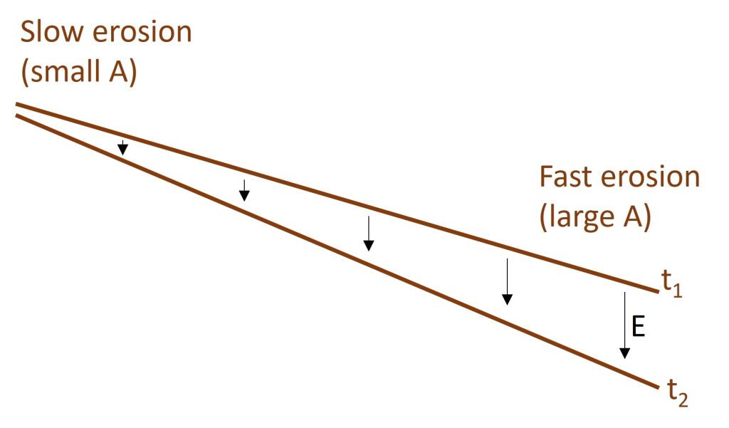
For example, consider an initially flat bedrock surface that is tilted by tectonic processes. The initial surface could be a wave-cut platform that is then tilted and uplifted by an earthquake (Fig. 1).

As runoff flows down this tilted surface and starts to carve a channel, how will the shape of the channel change over time? Specifically, how will the longitudinal profile of the channel evolve?

Based on eq. (2), since the surface initially has the same slope everywhere, slope alone will contribute to a background erosion rate that is constant along the profile. However, drainage area increases in the downslope direction, so drainage area alone will initially contribute to an erosion rate that increases in the downslope direction.

In other words, as the channel begins to erode, we expect the downstream end of the channel to erode faster than the upstream end.  At a later time, noted as [latex]t_2[/latex], the simple model predicts that the channel should look something like this (Fig. 2):

With just a little bit of erosion, it may not be clear whether the profile retains a constant (but steeper) slope, becomes concave (decreasing slope with distance), or becomes convex (increasing slope with distance).

Dynamic equilibrium

However, the concept of dynamic equilibrium can shed light on this. Dynamic equilibrium is the tendency for landscapes to change their form over time in a way that allows them to reach steady state, in which the erosion rate is constant everywhere. If dynamic equilibrium were not commonplace, landscapes would often experience runaway erosion that increases toward infinity over time, which isn’t so reasonable. Put another way, most geomorphic processes have some type of built-in negative feedbacks that tend to prevent runaway erosion, at least over long timescales.

If we treat [latex]E[/latex] as a constant to model dynamic equilibrium and rearrange eq. (2), we can see that there should be an inverse relationship between slope and area:

This means that for erosion rate to be constant everywhere along the profile, slope and drainage area should covary. Where drainage area is low, slope should be high, and where drainage area is high, slope should be low. Therefore, as the channel continues eroding, it should attain a convex form, illustrated at an even later time, [latex]t_3[/latex] below (Fig. 3).

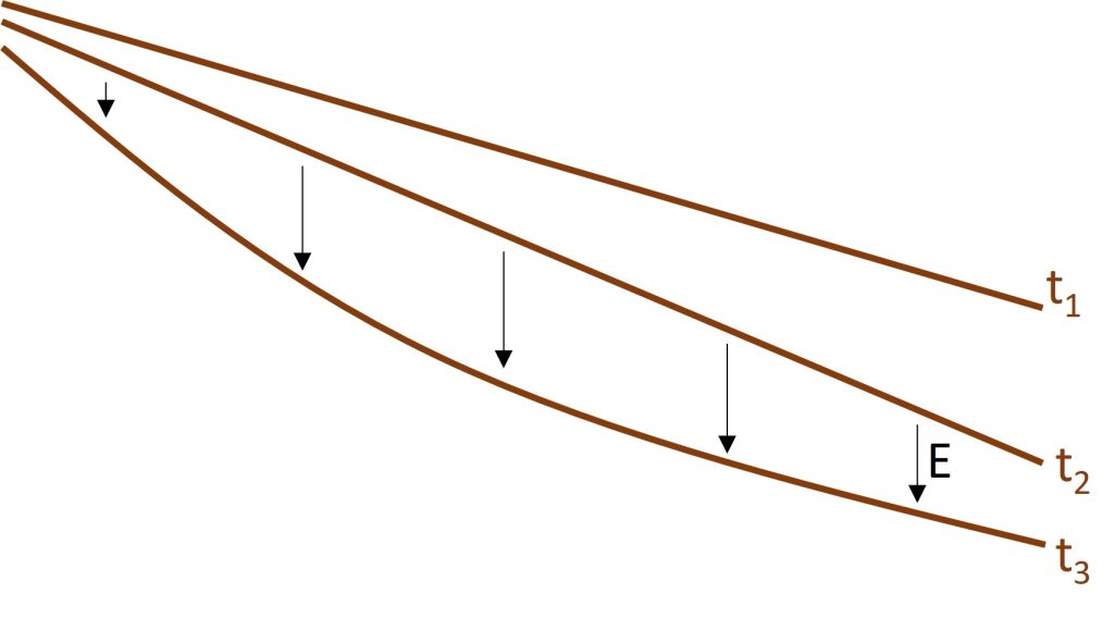
This inverse relationship between slope and drainage area and the resulting concave longitudinal profile is a fundamental characteristic of rivers. Rivers tend to be steep in their headwaters where they cascade out of mountain ranges and gentle at their mouths where they enter the oceans.

Exceptions

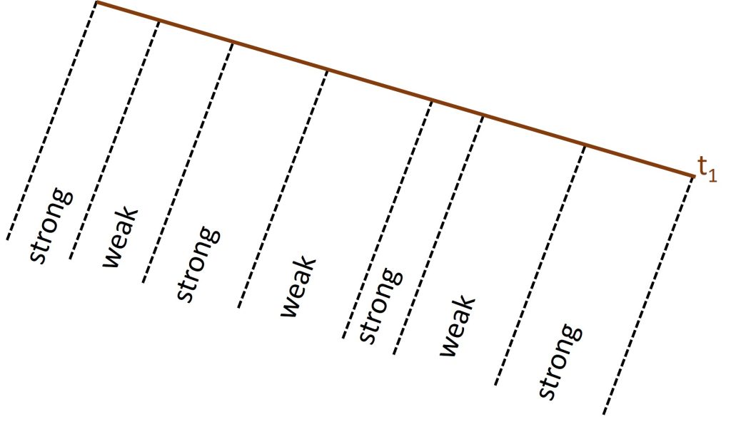
However, there are certainly exceptions to this general rule, like rapids or even waterfalls between gentler reaches of a river. Exceptions like this don’t invalidate the simple model, and can in fact be incorporated into the model by adding complexity. For example, let’s allow the erodibility constant, [latex]K[/latex], to vary in space.

Consider the same tilted bedrock surface as above, but now let’s assume it’s underlain by alternating layers of strong and weak sedimentary bedrock with a steep dip (Fig. 4). How does this change the development of the longitudinal profile?

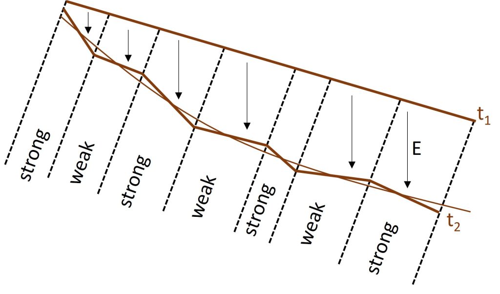
What happens to the slopes of two adjacent weak and strong layers as they erode? Since the layers are right next to each other, the drainage area is approximately the same for both layers. Furthermore, invoking dynamic equilibrium again, the erosion rate of both layers should be the same once the profile reaches steady state.

So if [latex]A[/latex] and [latex]E[/latex] are constant, slope should vary inversely with erodibility (eq. (3)). The stronger layers with large [latex]K[/latex] values should have steeper slopes, while the weaker layers with small [latex]K[/latex] values should have gentler slopes (Fig. 5).

This is telling us that steep slopes are required to erode strong rocks, while only gentle slopes are required to erode weak rocks at the same rate. So the weaker and stronger layers create local steps in the longitudinal profile, while the overall profile still has a generally concave form (because of the inverse relationship between slope and drainage area described above).

Overall, this vignette has shown that even a deliberately oversimplified model for a geomorphic process can be useful for conceptualizing the fundamental ways that process works. We will be deriving and using more complex models for erosion caused by different geomorphic processes throughout the rest of this book, and you’ll notice aspects of this very simple equation in each of them.