Theory

Flow of water through the subsurface is driven by changes in hydraulic head, which is defined as the energy per unit weight of the water. For slow movement of groundwater through the pore spaces in rocks and soils, gravitational potential energy is the most important type of energy that drives flow. Considering a small “parcel” of water in the subsurface, its potential energy is

and its weight is

where [latex]E[/latex] is gravitational potential energy [M L² T^-2], [latex]g[/latex] is acceleration due to gravity [L T^-2], [latex]h[/latex] is vertical elevation above a reference point [L], and [latex]W[/latex] is weight [M L T^-2].

Dividing eq. (1) by eq. (2) gives us the energy per unit weight. Since [latex]m[/latex] and [latex]g[/latex] cancel, the parcel of water’s hydraulic head is just [latex]h[/latex], its elevation above a reference point.

So, for unconfined aquifers, the most common type of aquifer we encounter near the earth’s surface, we usually assume that the height of the water table is equal to the hydraulic head at that location.

Numerous physical experiments that involve measuring the steady-state discharge of water through a sediment-filled tube under various head differences from one end of the tube to the other have shown that discharge increases linearly with the change in head, inversely with the length of the tube, and linearly with the cross-sectional area of the tube, all else being equal.

Putting these relationships together into one empirical equation gives us Darcy’s Law, which models the flow of water through porous media, such as rock and soil:

The last term in eq. (3), [latex]Δh/Δx[/latex], is also known as the head gradient. As the horizontal distance over which we measure the change in head becomes infinitesimally small, it becomes the derivative of [latex]h[/latex] with respect to [latex]x[/latex] in one dimension ([latex]dh/dx[/latex]) or more generally the gradient of [latex]h[/latex] ([latex]∇h[/latex]).

Also note the negative sign in eq. (3); this indicates that the direction of flow is opposite the head gradient. For example, if [latex]h[/latex] is increasing the to right, [latex]Δh/Δx[/latex] is positive, so [latex]Q[/latex] will be negative, i.e. to the left. Put simply, water flows downhill.

In addition to knowing the head gradient and cross sectional area of the aquifer we are interested in, we must determine a value for the hydraulic conductivity to determine discharge. This parameter generally captures how easily water moves through the medium. It varies by many orders of magnitude among different material types and depends on porosity, how connected that porosity is, and the spatial scale over which it is measured. It can be measured in the laboratory by forcing water to flow through a sample under different head gradients. Rearranging eq. (3) gives

so plotting [latex]Q/A[/latex] against [latex]Δh/Δx[/latex] should give points that lie on a straight line that goes through the origin, the slope of which will be the hydraulic conductivity, [latex]K[/latex].

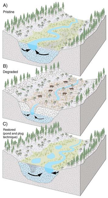
Case study: California Wet Meadows

For this case study, read the vignette on California wet meadows (e.g., Fig. 1). In these wet meadows, groundwater flows laterally through the soil underlying the floodplain toward a central stream. The elevation of that stream is the hydraulic head at that point, so changes in stream elevation over time change the head gradient in the vicinity (Fig. 2), which in turn affects groundwater discharge.

How can we estimate the hydraulic conductivity of these wet meadows at the field scale?

Example: Estimating hydraulic conductivity at the field scale

If we make a few simplifying assumptions and capitalize on a convenient rainfall event, we can roughly estimate the hydraulic conductivity of a wet meadow. In cross-section, first assume the floodplain soil has a uniform thickness of [latex]z[/latex] = 3 m and that it dips at a constant gradient of 0.03 m/m toward the stream (Fig. 3).

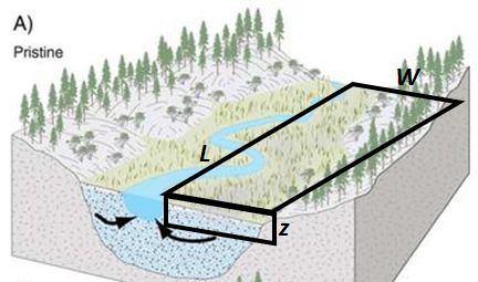
In mapview, assume one side of the floodplain can be approximated by a rectangle with a length, [latex]L[/latex] = 300 m, along the stream and a width, [latex]W[/latex] = 70 m, perpendicular to the stream.

During a long and steady rainstorm with average rainfall rate of [latex]P[/latex] = 0.2 cm/hr, the floodplain just becomes fully saturated. We can therefore reasonably assume that the head gradient is the same as the average floodplain dip, and more importantly that the volume of water infiltrating the floodplain from precipitation is about the same as the discharge of groundwater to the stream at its bank:

[latex]Q_r=Q_g[/latex],

(5)

where [latex]Q_r[/latex] is the vertical volumetric flux of rain water into the soil and [latex]Q_g[/latex] is the lateral volumetric flux of groundwater to the stream.

Since precipitation rate is in units of length per time, we need to multiply it by the area over which it is falling to get its volumetric flux:

[latex]Q_r=PLW[/latex].

(6)

The groundwater flux is determined by Darcy’s Law, with the relevant cross-sectional area being that of the floodplain soil at the stream bank, [latex]Lz[/latex], so we can set eq. (6) equal to eq. (3),

[latex]PLW=KLz\frac{Δh}{Δx}[/latex],

(7)

noting that the negative sign was dropped for simplicity and to deal only with magnitudes of these fluxes. Now, rearrange to isolate [latex]K[/latex], noting that [latex]L[/latex] cancels:

[latex]K=\frac{PW}{z}\frac{Δx}{Δh}[/latex].

(8)

Substituting in the values given above,

[latex]K=\frac{(0.2 cm/hr)(70 m)}{(3 m)}\frac{(1)}{(0.03)}=156 cm/hr[/latex],

so the hydraulic conductivity is on the order of a meter per hour, typical of rather sandy soils.